In this practical we begin by walking-through a simple example of MANOVA.
You’ll then have the opportunity to apply a MANOVA on a different dataset.
We’ll also walk-through an example of MANCOVA, which will include exploring the influence of covariates on group-based differences on multiple outcome variables.
Finally, you’ll have the opportunity to apply a MANCOVA on a different dataset.
37.2 MANOVA: demonstration
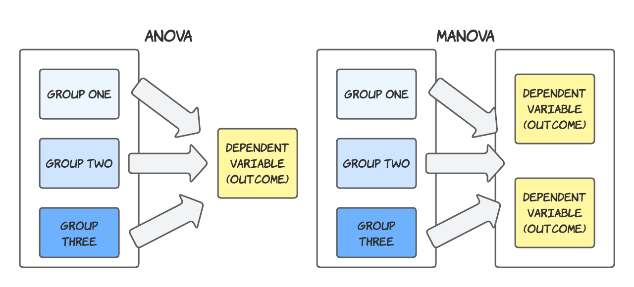
You’ll remember that MANOVA is used when we want to identify group (or sample) based differences in two or more dependent variables. It extends the principle of ANOVA, which can only deal with one dependent variable.
Load data
First, we’ll create a dataframe df by downloading a .csv file.
rm(list=ls())df <-read.csv('https://www.dropbox.com/scl/fi/jjh1sohgsv590f04x75pv/29_01.csv?rlkey=vhlxu0pziwymec3n7fiki2x1x&dl=1')head(df) # display the first six rows
In this dataframe, each observation (row) represents an athlete. We can see that each athlete has been allocated to one of three training programs (A, B or C).
This is the independent variable: the group to which the athlete has been allocated.
We can also see that their performance on three different outcome variables has been measured (sprint_time, jump_height, and throw_distance).
These are the dependent variables: the outcome measures we have collected.
Explore the Data
It’s always good practice to explore our data before we begin any complicated analyses.
In this case, we’re particularly interested in what the means of each group look like, for each of our three dependent variables.
We can use the dplyr package to examine differences in the mean of each outcome variable by group.
We can immediately see that there are between-group differences in the means for all the dependent variables. For example, athletes in Program_A have a lower mean sprint_time than those in Program_B.
We could also create some visuals to help explore the data:
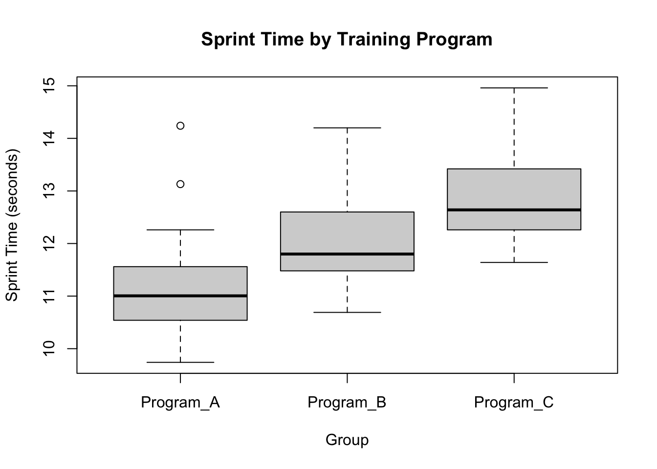
# Sprint Time Boxplotboxplot(sprint_time ~ training_program, data = df,main ="Sprint Time by Training Program",xlab ="Group", ylab ="Sprint Time (seconds)")
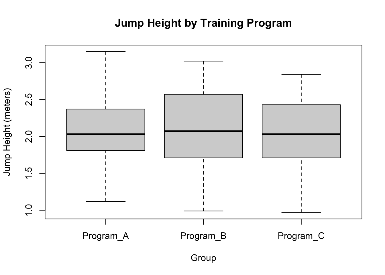
# Jump Height Boxplotboxplot(jump_height ~ training_program, data = df,main ="Jump Height by Training Program",xlab ="Group", ylab ="Jump Height (meters)")
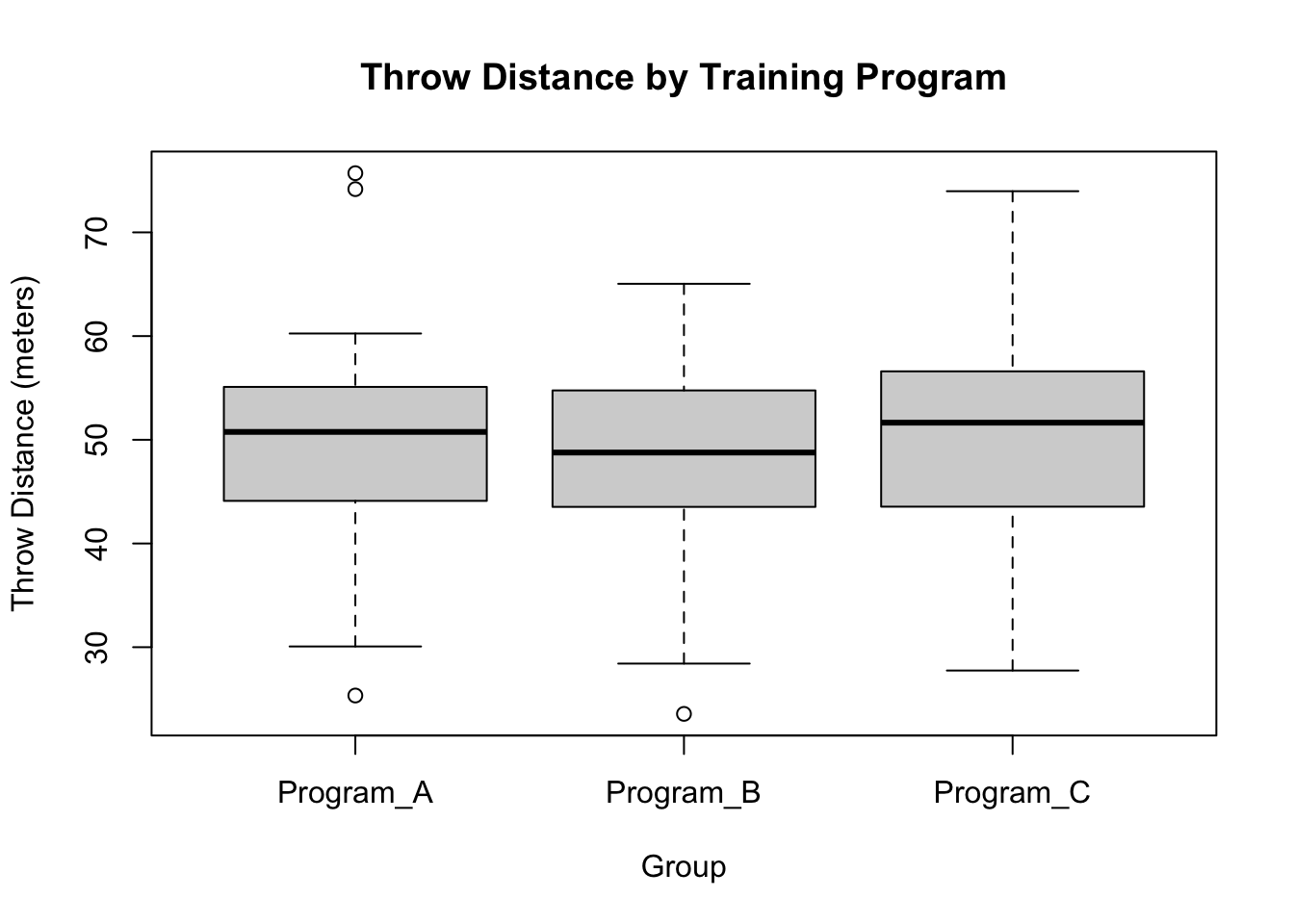
# Throw Distance Boxplotboxplot(throw_distance ~ training_program, data = df,main ="Throw Distance by Training Program",xlab ="Group", ylab ="Throw Distance (meters)")
These boxplots confirm what we saw earlier. It looks like athletes in Program A have a lower sprint_time than the other groups. However, we can’t yet say with confidence that these differences are significant (i.e., meaningful).
We need a statistical test to see if these differences are ‘real’.
Run MANOVA
We’re now ready to examine the effect of our independent variable, training_program, on the three dependent variables (sprint_time, jump_height and throw_distance).
Remember, we are hypothesising that an athlete’s performance on each of these variables depends on which level of the independent variable they belong to.
Here’s the R code to run the MANOVA:
# Conduct MANOVAmanova_fit <-manova(cbind(sprint_time, jump_height, throw_distance) ~ training_program, data = df)# Get summary of the MANOVAsummary(manova_fit)
 Response sprint_time :
                 Df Sum Sq Mean Sq F value    Pr(>F)
training_program  2 51.420 25.7098  29.255 1.143e-10 ***
Residuals        97 85.244  0.8788
---
Signif. codes:  0 '***' 0.001 '**' 0.01 '*' 0.05 '.' 0.1 ' ' 1

 Response jump_height :
                 Df  Sum Sq Mean Sq F value Pr(>F)
training_program  2  0.0734 0.03672  0.1467 0.8638
Residuals        97 24.2867 0.25038

 Response throw_distance :
                 Df  Sum Sq Mean Sq F value Pr(>F)
training_program  2   108.3  54.158  0.4995 0.6084
Residuals        97 10516.3 108.416
The second line of the output (starting with ‘training_program’) suggests that there are some significant between-group differences on at least one of the outcome variables. Notice the three *’s at the end of the line, which indicates p < 0.001.
In other words, athletes in different training programmes (A,B and C) appear to perform significantly differently on at least one outcome.
However, these first lines tell us nothing about the nature of that difference, or where it occurs.
Note
At this point, if you weren’t seeing a significant result in this first part of the output, you’d conclude that there are no significant differences as a result of training programme on any of the dependent variables.
As we have found a significant overall result, we need to explore this further.
The second part of our output tells us where those differences lie: it is in sprint time, as we suspected (again, notice the *’s indicating significance for this dependent variable).
So there are significant group-based differences for sprint time, but not for jump height (p>0.1) or training program (p>0.1).
Tukey’s ‘Honestly Significant Difference’ (HSD)
If we find a significant between-group difference for one or more of our dependent variables, we would typically use pairwise comparisons to examine the differences between levels of the independent variable for each dependent variable.
Remember, at this point, we don’t know which groups are significantly different from each other.
One common approach is to use Tukey’s Honestly Significant Difference (HSD) test. This test controls for the family-wise error rate when conducting multiple pairwise comparisons.
Notice that I’m only doing this for sprint_time, because we already know there are no significant differences between groups for our other dependent variables.
What is family-wise error rate?
FWER refers to the probability of making one or more false discoveries, or Type I errors, when performing multiple hypothesis tests simultaneously.
It’s the likelihood of incorrectly rejecting at least one true null hypothesis in a set of comparisons. Controlling the FWER is crucial in studies involving multiple comparisons to ensure the reliability of results, as it helps to maintain the overall error rate at a desired level, thereby reducing the chance of drawing incorrect conclusions from the data.
# Load necessary librarieslibrary(dplyr)library(multcomp)# Conducting Post-Hoc Tests# Tukey's HSD for Sprint_Timetukey_sprint <-TukeyHSD(aov(sprint_time ~ training_program, data = df))print("Tukey's HSD for Sprint_Time:")
[1] "Tukey's HSD for Sprint_Time:"
print(tukey_sprint)
  Tukey multiple comparisons of means
    95% family-wise confidence level

Fit: aov(formula = sprint_time ~ training_program, data = df)

$training_program
                         diff       lwr      upr     p adj
Program_B-Program_A 0.9771569 0.4318958 1.522418 0.0001364
Program_C-Program_A 1.7471569 1.2018958 2.292418 0.0000000
Program_C-Program_B 0.7700000 0.2206849 1.319315 0.0034206
This output confirms significant between-group differences for all training programmes on sprint time. In each case, p < 0.01.
We can go back to our table of means to interpret this; Program A had a mean sprint time of 11.1, B had a mean of 12.1 and C had a mean of 12.9.
Athletes in A had a significantly better performance than those in B and C, and athletes in B had a significantly better performance than those in C.
Therefore, at the end of our analysis, we can conclude that the training programs had a significant effect on an athlete’s sprint time, but had no significant effect on their jump height or throw distance.
I wonder if you can reflect on why this might be useful within an applied sport data analytics situation? What could you do with such information?
37.3 MANOVA: Practice
Using the data file available at the following link, repeat the analysis above. Take time to examine the data before undertaking the MANOVA.
Download the datafile and create a new dataframe. Explore the dataframe to determine what it represents.
Conduct some exploratory analysis of the data, including group-based differences.
Conduct a MANOVA to examine whether there are any significant differences in the dependent variables between groups.
If you find there are, explore your model further to determine where those differences lie.
If you identify significant differences, utilise Tukey’s HSD to pinpoint where those differences are found.
Show solution
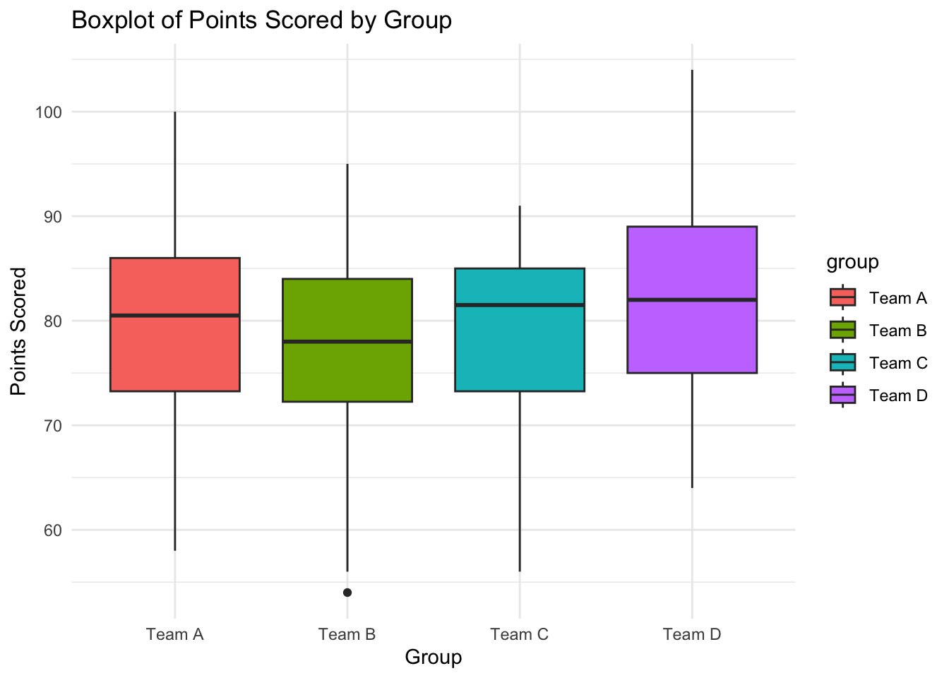
#----------------------# data loading#----------------------df_2 <-read.csv('https://www.dropbox.com/scl/fi/3d5itbmyp5wgqbkajhctm/basketball_dataset.csv?rlkey=6wrmvey8uhvu67egh8g8twnmr&dl=1')#----------------------# data preparation#----------------------df_2$X <-NULLstr(df_2)
#----------------------# data visualisation#----------------------library(ggplot2)# Boxplot for points scored by groupggplot(df_2, aes(x = group, y = points_scored, fill = group)) +geom_boxplot() +labs(title ="Boxplot of Points Scored by Group",x ="Group",y ="Points Scored") +theme_minimal()
Show solution
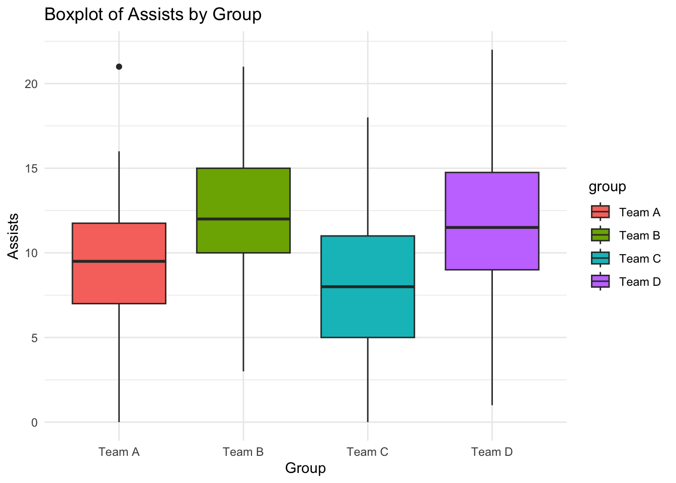
# Boxplot for assists by groupggplot(df_2, aes(x = group, y = assists, fill = group)) +geom_boxplot() +labs(title ="Boxplot of Assists by Group",x ="Group",y ="Assists") +theme_minimal()
Show solution
#----------------# Conduct MANOVA#-----------------manova_fit <-manova(cbind(points_scored, assists) ~ group, data = df_2)# Get summary of the MANOVAsummary(manova_fit)
           Df  Pillai approx F num Df den Df    Pr(>F)
group       3 0.17806    6.385      6    392 1.982e-06 ***
Residuals 196
---
Signif. codes:  0 '***' 0.001 '**' 0.01 '*' 0.05 '.' 0.1 ' ' 1
Show solution
summary.aov(manova_fit) # For univariate effects
 Response points_scored :
             Df  Sum Sq Mean Sq F value Pr(>F)
group         3   551.6 183.880  1.9175  0.128
Residuals   196 18795.1  95.893

 Response assists :
             Df Sum Sq Mean Sq F value    Pr(>F)
group         3  656.0 218.672  10.935 1.133e-06 ***
Residuals   196 3919.6  19.998
---
Signif. codes:  0 '***' 0.001 '**' 0.01 '*' 0.05 '.' 0.1 ' ' 1
Show solution
#------------------# Explore group-based differences using Post-Hoc tests# Load librarieslibrary(multcomp)# Tukey's HSD for Sprint_Timetukey_assists <-TukeyHSD(aov(assists ~ group, data = df_2))print("Tukey's HSD for Assists:")
[1] "Tukey's HSD for Assists:"
Show solution
print(tukey_assists)
  Tukey multiple comparisons of means
    95% family-wise confidence level

Fit: aov(formula = assists ~ group, data = df_2)

$group
               diff         lwr        upr     p adj
Team B-Team A  3.18  0.86247773  5.4975223 0.0026452
Team C-Team A -1.34 -3.65752227  0.9775223 0.4405080
Team D-Team A  2.38  0.06247773  4.6975223 0.0416409
Team C-Team B -4.52 -6.83752227 -2.2024777 0.0000059
Team D-Team B -0.80 -3.11752227  1.5175223 0.8077275
Team D-Team C  3.72  1.40247773  6.0375223 0.0002771
37.4 MANCOVA: Demonstration
The purpose of MANCOVA is to include an analysis of the effects of potential covariates in our data.
Step One: Load data
First, I’m going to clean the environment and re-load the first dataset.
rm(list=ls())df <-read.csv('https://www.dropbox.com/scl/fi/xe2n37vfyck76i7hw4gnn/mancova_cycling.csv?rlkey=1khog9n5p1sh9evgsi6ovr5ta&dl=1')df$X <-NULLhead(df) # display the first six rows
In this cycling-based dataset, we have a similar structure to the previous dataset. There is a training_program (the IV, which is Program A or Program B) and a series of DVs (speed. elevation and time). We also have the athlete’s age.
We’re going to carry out a similar analysis to the previous one, asking the question “does training program have a significant effect on performance on any of the three dependent variables”? This time, we’re going to include age as a covariate, because it’s reasonable to suspect that it might be influential in how training program impacts performance.
Step Two: Examine potential interactions
When we conducted the MANOVA analysis above, we ignored the age variable. All we were interested in was whether the training program had a significant effect on any of the outcome variables.
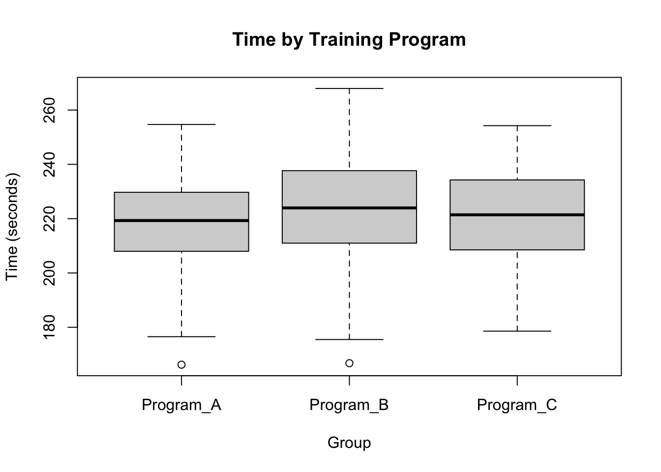
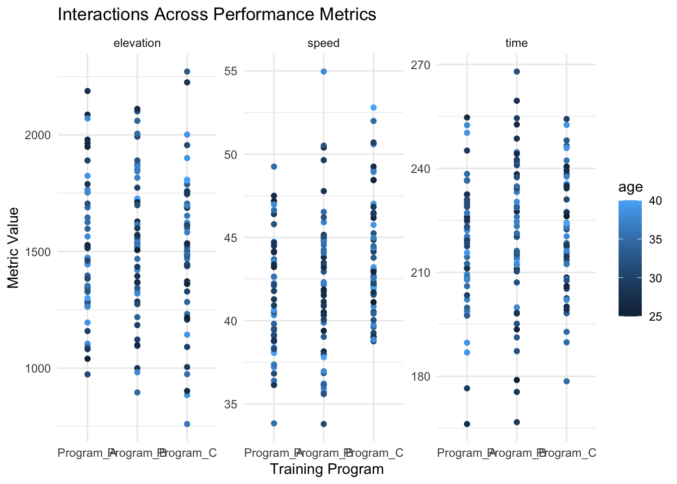
We can visually inspect the impact of DV on the IVs:
# Time Boxplotboxplot(time ~ training_program, data = df,main ="Time by Training Program",xlab ="Group", ylab ="Time (seconds)")
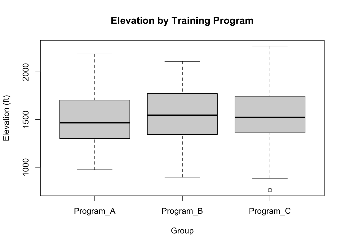
# Elevation Boxplotboxplot(elevation ~ training_program, data = df,main ="Elevation by Training Program",xlab ="Group", ylab ="Elevation (ft)")
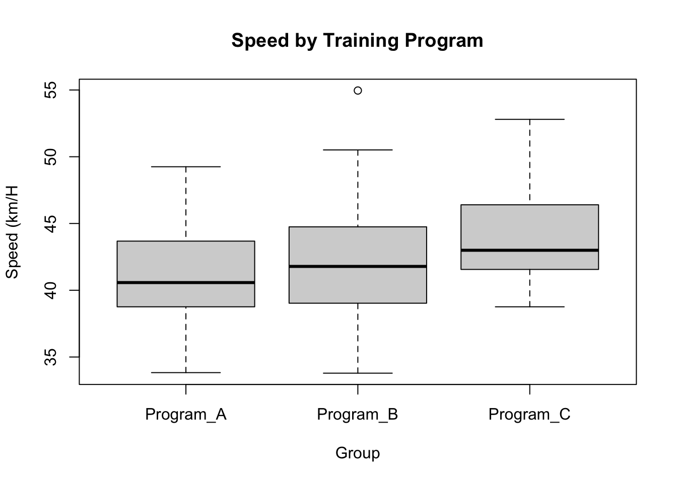
# Speed Boxplotboxplot(speed ~ training_program, data = df,main ="Speed by Training Program",xlab ="Group", ylab ="Speed (km/H")
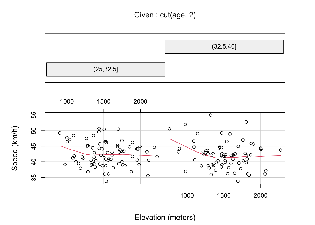
But it’s reasonable to assume that age might also be important in this association. That is where MANCOVA becomes useful; we want to examine covariates of our main predictor variable, in this case age.
Reminder: what’s a covariate?
A ‘covariate’ is a variable that is possibly predictive of the outcome under study (the dependent variable). In statistics, covariates can be ‘controlled’, which lets us isolate the effect of the primary variable(s) of interest (the independent variable/s).
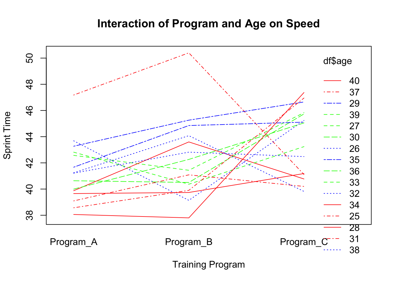
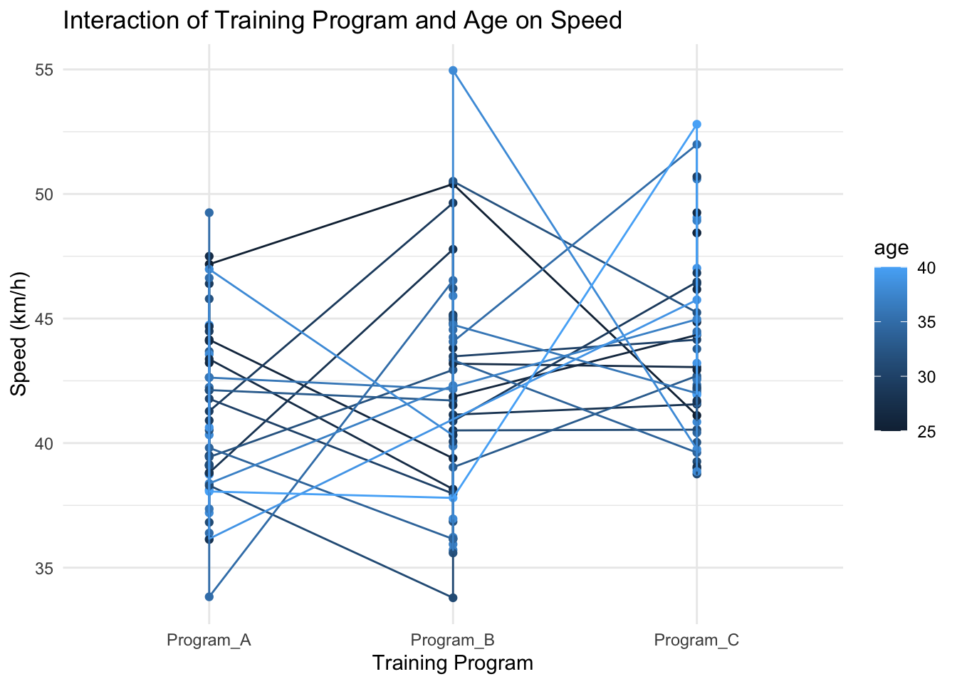
Interaction plots are useful for visualising how the relationship between one independent variable and a dependent variable changes across levels of another independent variable or covariate.
# Interaction of Program, Age, and Speedinteraction.plot(df$training_program, df$age, df$speed,main="Interaction of Program and Age on Speed",xlab="Training Program", ylab="Sprint Time", col=c("red","blue","green"))
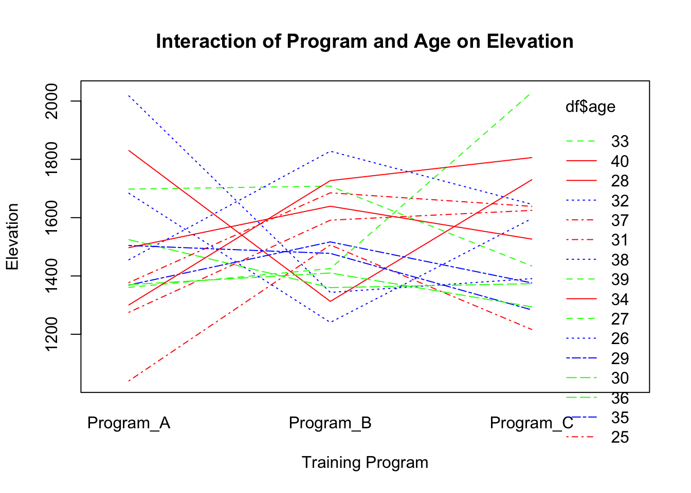
# Interaction of Program, Age, and Elevationinteraction.plot(df$training_program, df$age, df$elevation,main="Interaction of Program and Age on Elevation",xlab="Training Program", ylab="Elevation", col=c("red","blue","green"))
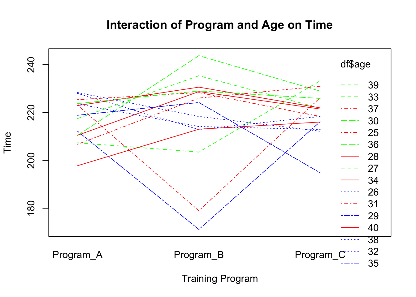
# Interaction of Program, Age, and Timeinteraction.plot(df$training_program, df$age, df$time,main="Interaction of Program and Age on Time",xlab="Training Program", ylab="Time", col=c("red","blue","green"))
Here are some other ways you can visualise interaction effects:
library(ggplot2)# Interaction plot for Speed as a function of Training Program and Ageggplot(df, aes(x=training_program, y=speed, color=age)) +geom_point() +geom_line(aes(group=age)) +theme_minimal() +labs(title="Interaction of Training Program and Age on Speed",y="Speed (km/h)",x="Training Program")
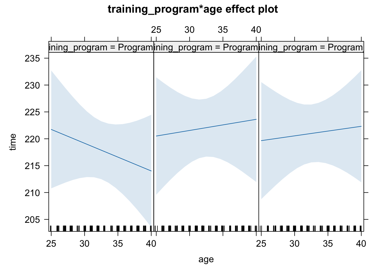
# Fit a linear model for demonstrationmodel <-lm(time ~ training_program * age, data = df)# Create interaction plots based on model predictionslibrary(effects)plot(allEffects(model))
Step Three: MANCOVA
The following example uses the the manova function from R’s base statistical package.
This lets us analyse the influence of training_program on our dependent variables while controlling for the effects of age, which is our covariate.
The command mancova_fit <- creates a new variable named mancova_fit that will store the results of the MANCOVA analysis.
The command manova() calls the function to perform the multivariate analysis of variance (MANOVA).
Note that the model specification is different from the MANOVA conducted above. This time, we’ve included a covariate (age), which makes the analysis a MANCOVA.
The command cbind(sprint_time, jump_height, throw_distance) specifies the dependent variables for the analysis, binding them together into a multivariate response. Here, sprint_time, jump_height, and throw_distance are the dependent variables being analysed.
~ separates the dependent variables from the independent variables and covariates in the formula.
training_program + age specifies the independent variable (training_program) and the covariate (age). The training_program variable is what the analysis aims to examine in terms of its effect on the three dependent variables, while age is included as a covariate to control for its potential confounding effect, allowing for a more accurate assessment of the impact of training_program.
# MANCOVA model with Age as a covariatemancova_fit <-manova(cbind(time, elevation, speed) ~ training_program + age, data = df)# Viewing the Resultssummary(mancova_fit)
 Response time :
                  Df Sum Sq Mean Sq F value Pr(>F)
training_program   2    495  247.53  0.6780 0.5092
age                1      8    7.81  0.0214 0.8839
Residuals        146  53303  365.09

 Response elevation :
                  Df   Sum Sq Mean Sq F value Pr(>F)
training_program   2    39282   19641  0.2105 0.8104
age                1       63      63  0.0007 0.9793
Residuals        146 13621890   93301

 Response speed :
                  Df  Sum Sq Mean Sq F value   Pr(>F)
training_program   2  200.97 100.483  6.7063 0.001635 **
age                1   16.91  16.909  1.1285 0.289845
Residuals        146 2187.57  14.983
---
Signif. codes:  0 '***' 0.001 '**' 0.01 '*' 0.05 '.' 0.1 ' ' 1
Step Four: Interpretation
The MANCOVA output provides information on how the independent variables (both the grouping variable and the covariate) affect the combined dependent variables, controlling for the effects of the covariates.
On the first line of the output, we can see that training program membership has a signficant effect on at least one of the dependent variables.
However, age does not seem to be a significant covariate. Pillai’s Trace is a good general-purpose test. A significant p-value indicates that there is a statistically significant difference in the combined dependent variables across the groups, after controlling for the covariate(s).
In the example above, the p-value for Pillai’s Trace is > 0.05, which suggests that, overall, age does not play a significant role in the association between training program membership and any of the dependent variables.
Moving down, we can see that training program has a significant effect on speed. age is not significant, confirming that it does not play any role in mediating the relationship between program membership and speed.
Multiple Comparisons: If you further explore specific group differences with post-hoc tests, remember to adjust for multiple comparisons to control the Type I error rate.
37.5 MANCOVA: Practice
Re-load the first dataset.
rm(list=ls())df <-read.csv('https://www.dropbox.com/scl/fi/jjh1sohgsv590f04x75pv/29_01.csv?rlkey=vhlxu0pziwymec3n7fiki2x1x&dl=1')df$X <-NULLhead(df) # display the first six rows
Now, conduct a MANOVA that explores whether age is a significant covariate on any of the outcome variables (sprint_time, jump_height, throw_distance).
You should be able to report:
Whether training program has any significant impact on any of the outcome variables.
Whether any of these findings (significant or insignificant) appear to be affected by the athlete’s age.
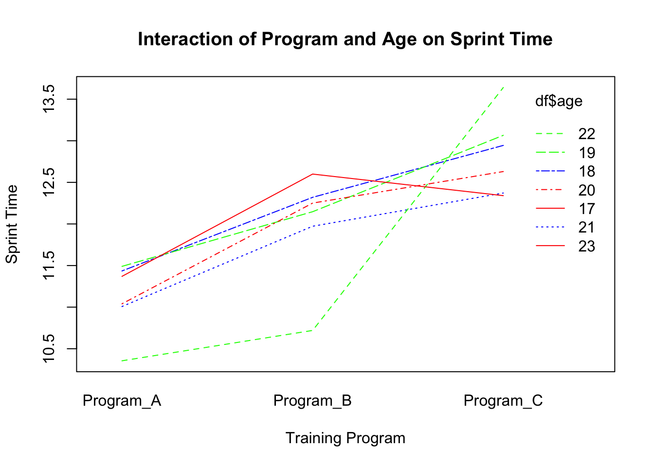
#| code-fold: true#| code-summary: Show solution# Interaction of Program, Age, and Sprint_Timeinteraction.plot(df$training_program, df$age, df$sprint_time,main="Interaction of Program and Age on Sprint Time",xlab="Training Program", ylab="Sprint Time", col=c("red","blue","green"))
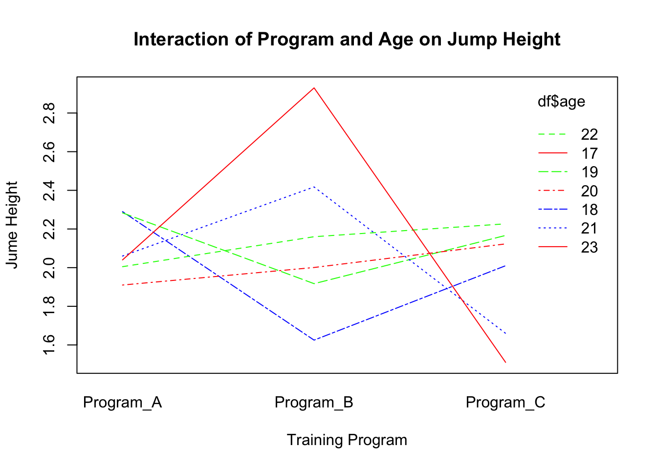
# Interaction of Program, Age, and Jump_Heightinteraction.plot(df$training_program, df$age, df$jump_height,main="Interaction of Program and Age on Jump Height",xlab="Training Program", ylab="Jume Height", col=c("red","blue","green"))
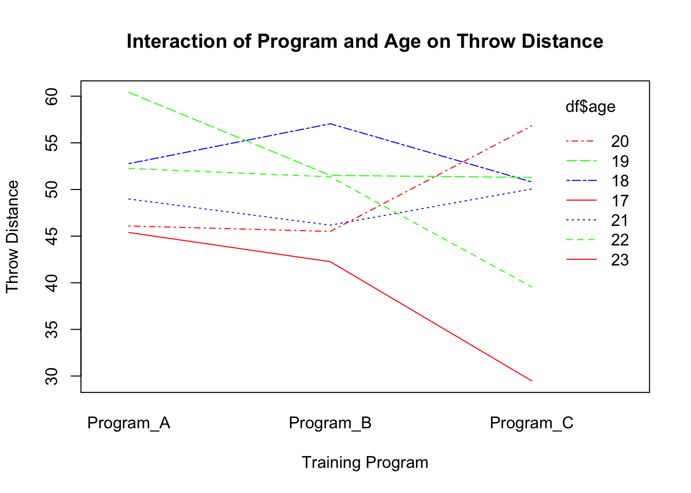
# Interaction of Program, Age, and Throw_Distanceinteraction.plot(df$training_program, df$age, df$throw_distance,main="Interaction of Program and Age on Throw Distance",xlab="Training Program", ylab="Throw Distance", col=c("red","blue","green"))
### MANCOVA# MANCOVA model with Age as a covariatemancova_fit <-manova(cbind(sprint_time, jump_height, throw_distance) ~ training_program + age, data = df)# Viewing the Resultssummary(mancova_fit)